

Two-Dimensional Gabor-Granger: When Your Pricing Problem Has Two Moving Parts

Pricing research has a reputation for being resource heavy and analytically heavy. Some studies earn that reputation. Many don’t need to. Rajan Sambandam’s framework for practical pricing research lays out the gamut of available methods, and plenty of them are simple survey exercises that capture preference at a handful of price points. (Our paper on monadic designs versus price laddering covers two of them.) It’s when you have several variables to test alongside price that you land on conjoint analysis, with the budget and timeline that matches the increased complexity.
But what if you only have two variables? A method we’ve developed at TRC says you can still get where you’re going without a conjoint, by extending a pricing technique that’s been trusted for sixty years.
The Pricing Research Challenge: When Price Depends on Another Variable
Suppose you’re the insights lead at a payments company. The company processes payments for merchants, charges a fee on each transaction, and deposits the remaining funds into the merchant’s account. The team responsible for merchant pricing comes to you with a question: What transaction fee should we charge?
At first, this looks easy. Test a few fee levels in a survey, find where merchants start walking away, and you’re done. You’re thinking a simple price ladder or Gabor-Granger exercise. A few weeks of work.
Then the product manager sits in on the kickoff, and the question gets more complicated. The fee can’t be tested on its own because it’s tied to a second variable: how quickly merchants get access to their funds. Some merchants will happily pay less and wait longer. Others need the money immediately and are willing to pay more for faster access. Picture a large merchant with sufficient cash reserves that can afford to wait, compared with a small business trying to cover payroll that week. Determine the right fee without considering how quickly funds become available, and you’ve answered only half the question.
So now you have a problem. The standard playbook points to conjoint analysis, and that means a bigger study: more design work, more programming, a model to estimate, and a set of outputs you’ll have to explain to stakeholders. The budget and timeline both climb, and you’re the one who has to go back and explain why the simple study stopped being simple.
But you only have two variables, not six. That’s a specific situation, and it has a specific answer. TRC’s two-dimensional Gabor-Granger approach (2D Gabor-Granger or 2D-GG) tests both variables in one straightforward survey and returns pricing curves for every payout speed. No utility modeling, no market simulator, and no technical estimates to explain to stakeholders. Let’s look at how it works and what our payments example produces.
How 2D Gabor-Granger Measures Price Tradeoffs
– Measuring Willingness to Pay Across Multiple Price and Attribute Combinations
Classic Gabor-Granger walks a respondent up and down a price ladder. Ask about a price, go higher and ask again if they’d buy, lower if they wouldn’t, and stop when you’ve found the most they’ll pay. 2D Gabor-Granger does the same thing in two dimensions at once. Instead of a ladder, you have a grid.
For our payments example, the hypothetical grid is five transaction fees (2.6%, 2.8%, 3.0%, 3.2%, and 3.4%) crossed with four payout speeds (same day, 1 day, 3 days, and 5 days). That’s twenty combinations. Each merchant answers a short sequence of accept-or-reject questions, and by the end, every one of those twenty combinations is marked acceptable or unacceptable for that merchant, in the units you actually price in.
The efficiency comes from a simple observation. If a merchant accepts 3.0% with a 1-day payout, they’ll also accept 2.8% with a 1-day payout, and 3.0% with a same-day payout, and anything else that’s better on both counts. Those cells fill in without being asked, as Figure 1 illustrates.
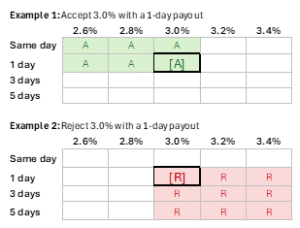
Figure 1. A single response determines multiple grid cells. Accepting a combination implies acceptance of all combinations that are better on both dimensions; rejecting a combination implies rejection of all combinations that are worse on both dimensions.
The same logic runs backwards: reject a combination and everything worse on both counts is rejected too. The survey only asks about combinations that are still genuinely open, and each answer settles several at once instead of just the one you asked about. In our example, a typical merchant answers about seven questions and the other thirteen cells follow from that better-on-both-counts assumption. It’s the same assumption behind any staircase pricing exercise, and it’s what creates the efficiency.
All the method needs is that each number has a consistent direction of preference. Lower fee is always better, faster payout is always better. Given that, the grid is yours to design around the decision you’re actually making. The levels you pick determine what you can see, so cover the range you might realistically act on. Any values between the tested levels are estimated from the curve rather than measured directly.
Here’s what a merchant would see. In this example each merchant judges one offer at a time:
Your payouts arrive 1 day after the sale, and you pay a 3.0% fee on each transaction. Would you sign up?
That’s it. Seven or so of those, with the numbers changing each time based on the previous answer. You can also run it against a fixed competitor offer instead of on its own, if that’s closer to the real decision, and the logic underneath is identical.
How many merchants do you need? Because there’s no advanced choice modeling involved, standard sample-size considerations for stated survey questions apply. Larger samples reduce the margin of error and allow for more reliable reads within individual audiences. The appropriate sample ultimately depends on the precision the decision requires and which audiences need to be analyzed separately.
Pricing Research Results: Demand Curves, Willingness to Pay, and Customer Tradeoffs
To illustrate the output, we simulated responses from 1,000 merchants. The numbers that follow are not findings about the payments market; they’re simply an example of what a completed 2D Gabor-Granger study might produce.
So what lands on your desk? The core output is a table showing the take rate at every fee-and-speed combination on your grid. Table 1 shows an example based on our simulated data.
Table 1. Merchant take rate by payout speed and transaction fee (simulated, N = 1,000).
| 2.6% | 2.8% | 3.0% | 3.2% | 3.4% | |
| Same day | 89% | 78% | 60% | 41% | 25% |
| 1 day | 86% | 72% | 51% | 32% | 16% |
| 3 days | 77% | 58% | 36% | 20% | 8% |
| 5 days | 64% | 43% | 22% | 10% | 3% |
Read across any row and you have a demand curve at a fixed payout speed. Read down any column and you have the response to payout speed at a fixed fee. Where a traditional price ladder gives you one demand curve, Table 1 gives you four (one for each payout speed).
Table 1 is the foundation for the rest of the analysis. Some questions can be answered directly from the table. Others, including merchants’ willingness to pay for faster access to their funds, are harder to see in a grid of numbers. Plot the same data, and the answer becomes clear.
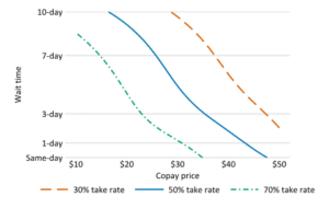
Figure 2. Every fee-and-speed combination that holds the same share of merchants. Simulated, N = 1,000.
Suppose you’re aiming to sign up half the merchants you approach. Figure 2 can be read at any target take rate, but we’ll use 50% as an example. The middle line shows every fee-and-speed combination that reaches that target. Follow it and the tradeoff is right there: same-day payout gets you to 50% acceptance at about 3.1%, while 5-day payout gets you there at about 2.8%. That gap answers the product manager’s question. Going from the slowest payout to the fastest is worth about a third of a percentage point in additional fees, which you can compare with the cost of funding same-day settlement.
Recall that in our simulation, each merchant answers only a subset of the grid, with the remaining cells filled in logically from those responses. The result is a complete grid for every merchant, which means you can analyze subgroups just as you analyze the full sample. Split the merchants by size, for example, and a meaningful difference emerges: smaller merchants, whose cash flow may be tighter, are willing to pay more for faster access to their funds than larger merchants with more cash on hand. To reach 50% acceptance for same-day payout, you could charge smaller merchants about 3.3%, compared with about 3.0% for larger merchants. That difference is less visible in the pooled result, but it gives the product manager actionable guidance on how to price, target, and position the offer.
So, back to where we started. The team responsible for merchant pricing asked you what fee to charge. The product manager pointed out that you couldn’t answer that without considering payout speed. The standard playbook said conjoint analysis. Instead, a 2D Gabor-Granger showed what each fee buys you at every payout speed, what faster access to funds is worth, and how differently large and small merchants value it. You got all of that from a survey that asked each merchant about seven questions.
Pricing Strategy Research Across Products, Services, and Industries
- Examples of Pricing Research Questions 2D Gabor-Granger Can Answer
We’ve used payments as our example, but this problem isn’t specific to payments. It arises whenever a decision depends on two numeric variables. The second variable isn’t always time. Sometimes it’s a quantity, and sometimes it’s a financial term. What these problems share isn’t an industry, but the need to price two related variables together.
Table 2. Examples of Two-Variable Pricing Decisions Across Industries
| Industry | Price attribute | Second attribute | The decision |
| Payments (our example) |
Transaction fee (%) | Days to payout | Fee against settlement speed |
| Health insurance | Monthly premium | Deductible | How much more per month to lower the deductible |
| Health provider | Price of self-pay service | Days to next appointment | What to charge for faster access |
| Banking | Mortgage interest rate | Upfront discount points | Rate against what you pay to buy it down |
| Prepaid cards | Monthly card fee | Days early for direct deposit | Fee against earlier access to pay |
| Telecom | Monthly price | Download speed | Price against speed |
| Streaming | Monthly price | Ad minutes per hour | Price against ad tolerance |
These are just a few examples. The common thread is a business that needs to understand the tradeoff between two numeric variables. The method fits when those two variables drive the decision and the rest of the offer remains fixed. Once a third attribute meaningfully affects the choice, conjoint analysis is likely the better approach, as the next section explains.
Choosing the Right Pricing Research Method: 2D Gabor-Granger vs classic Gabor-Granger vs Conjoint
- Use 2D Gabor-Granger when two quantitative attributes both drive the decision and both need to vary, each attribute has a consistent direction of preference (lower is always better, or higher is always better, either works), and what you need is the tradeoff between them: how acceptance moves across the grid, and what one attribute is worth in terms of the other.
- Use classic Gabor-Granger or Van Westendorp when only price is moving and no second attribute is material to the decision.
- Use conjoint when three or more attributes are actively varying, when categorical attributes are in play (brand, feature presence, service tier), when preferences aren’t monotonic (a middle level can be preferred over both extremes, the way people pick a screen size), or when you need share estimation across a realistic competitive set.
The narrowness is the point. 2D Gabor-Granger isn’t a replacement for conjoint. It is designed for a specific, common problem that is more than single-attribute methods can address but does not require the full machinery of conjoint.
Where 2D Gabor-Granger Fits Within a Broader Pricing Research Strategy
The two-variable problem keeps turning up in client briefs, and the usual answers have never been very satisfying. Either “that’s a conjoint,” which is true but heavier than the problem requires, or “let’s hold the second attribute fixed,” which is cheaper but answers the wrong question. We wanted a third answer. So 2D Gabor-Granger now sits alongside Gabor-Granger, Van Westendorp, brand price trade-off, and choice-based conjoint in our pricing practice.
Further reading. The full method, including the task selection logic, worst-case task counts by grid size, monadic and competitive deployment, and a runnable simulation script, is in the working paper on SSRN: Two-Dimensional Gabor-Granger: A Pricing Research Method for Two-Attribute Tradeoffs. A practitioner-oriented article on the method is also forthcoming in the November/December 2026 issue of Quirk’s Marketing Research Review.
Have a pricing problem with two moving parts? Talk to us about pricing research.
About the author
Westley Ritz is Vice President of Analytics at TRC Insights, where he leads the analytics team and TRC’s applied AI work in market research. He works primarily in choice modeling (conjoint, MaxDiff), pricing research, and segmentation, and co-developed TRC’s Two-Dimensional MaxDiff method. He holds an M.S. in Statistics from Temple University and a B.S. in Statistics and Economics from the University of Michigan.
The simulated data in this paper illustrates the form of the method’s output. It is not a finding about the payments market.